Get started with benchtm
a01_User_guidance.RmdR package “benchtm” can be used to generate data for the comparison of subgroup identification algorithms. To start with, we can directly load the library using:
Data Generation Framework
Consider a two-arm study where trt = 0 represents control arm and trt = 1 represents treatment arm, the clinical outcome/response \(Y\) is generated from
\[\begin{equation} \mathbb{E} (Y|X) = g(f(X)) = g(f_{prog}(X) + trt*(\beta_0 + \beta_1 f_{pred}(X))), \end{equation}\]
where \(g(\cdot)\) is the link
function and \(f_{prog}(X)\) is the
functional form of the prognostic variables and \(f_{pred}(X)\) is the functional form of the
predictive variables; \(\beta_0\) and
\(\beta_1\) are the coefficients of
main treatment effect and the predictive effects respectively. From the
data generation formula one can see that, the larger the \(\beta_0\), the more power there is to
detect the overall treatment effect. The parameter \(\beta_1\) determines the treatment effect
variability (increasing if \(|\beta_1|\) gets larger). Larger \(|\beta_1|\) implies that it is more likely
to detect the subgroup. \(\beta_0\) and
\(\beta_1\) together determine the
overall treatment effect. The function generate_y can be
used to generate the outcome values \(y\).
To generate the binary treatment variable, we consider \[P(trt = 1|X) = \frac{1}{1+\exp(-h(X))}\]
where \(h(X)\) is a user specified
form. When \(h(X) = 0\), \(P(trt = 1|X) = 0.5\) represents a setting
for complete randomized design (have a look at the function
generate_trt for details).
Depending on different types of responses, the link function \(g(\cdot)\) and how the clinical endpoints are generated are given as:
- Continuous response: \(g(x) = x\) and \(Y \sim N(\mu = g(f(X)), \sigma)\).
- Binary response: \(g(x) = \dfrac{e^x}{1 + e^x}\) and \(Y \sim \text{Bernoulli}(p = g(f(X)))\).
- Count response: \(g(x) = e^x\) and \(Y\sim \text{Poisson}(\lambda = g(f(X)))\).
- Time-to-event response: \(g(x) = e^x\) and \(t\sim \text{Exponential}(\lambda = g(f(X)))\).
Example of using ``benchtm’’ package
In this section we provide an example of using “benchtm” package to generate a dataset for subgroup identification problem.
For the covariates, one can either utilize a user-specified dataset
or generate them from the function generate_X_dist
(generate covariates from a pre-specified distribution) or
generate_X_syn (generate data from synthetic data from a
specific real trial). See each corresponding function for more
details.
set.seed(1111)
X <- generate_X_dist(n=1000, p=10, rho=0.5)
#observational data set
trt <- generate_trt(n=nrow(X), p_trt = 0.5)
dat <- generate_y(X, trt, prog = "0.5*((X1=='Y')+X3)",
                   pred = "X3>0", b0 = 0, b1 = 1,
                   type = "continuous", sigma_error = 3)

head(dat)
#>   trt X1         X2          X3          X4 X5 X6          X7         X8
#> 1   0  N 0.03125259  0.09421509  0.51514432  N M2 -0.98045591  0.1306782
#> 2   1  N 0.83737617 -1.09363394 -0.55371671  N M3  1.99750426  0.2235778
#> 3   0  Y 1.18467412  2.28562630  0.13729403  Y M1  1.59946889 -1.0619646
#> 4   0  N 1.87707398  0.93545962 -0.52007261  N M2  0.12848242  0.8768221
#> 5   1  Y 0.59686419  0.16525676  0.20060728  N M2 -0.08869092  0.9582106
#> 6   1  Y 2.00749871 -0.08007514  0.08383461  Y M3 -0.75252169  1.6078133
#>            X9        X10          Y
#> 1 -2.71313108  0.6942494  1.1067937
#> 2  0.87700756  1.0092612 -2.6188408
#> 3 -0.07447738 -0.1410665  3.6697095
#> 4 -0.11605592  0.4896499 -0.8245078
#> 5 -0.97397058  0.1617459  2.4050540
#> 6 -0.30708657  0.1690040  4.9389464
The treatment is generated based on randomized trial where \(P(trt = 1) = 0.5\). We could fit a conditional tree using this generated data.
cov.names <- dat %>% dplyr::select(starts_with("X")) %>% colnames()
eqn <- paste0("Y ~ trt| ",
              paste0(cov.names, collapse = "+"))

glmtr <- partykit::glmtree(as.formula(eqn), data = dat, family = "gaussian",
                           minsize = 0.2*nrow(dat))
plot(glmtr)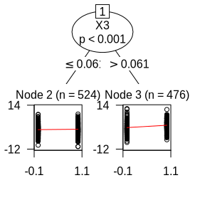
Based on the results, one can see that \(X_3\) is selected as the split variable. The subgroup with \(X_3>0.061\) has the largest treatment effect.